Examples

This page demonstrates how to use different bone spatial models and visualize their results. The requirement for running the models is the installation of the bone_models package via running the command pip install bone_models in the terminal.

Lerebours Model Example

from bone_models.bone_spatial_models.models.lerebours_model import Lerebours_Model
from bone_models.bone_spatial_models.load_cases.lerebours_load_cases import Lerebours_Load_Case_Spaceflight
import matplotlib.pyplot as plt
import numpy as np

load_case = Lerebours_Load_Case_Spaceflight()
model = Lerebours_Model(load_case, duration_of_simulation=4)

cross_section, results = model.solve_spatial_model()
y_coords = cross_section['y'].values * 1e3  # Convert to mm
z_coords = cross_section['z'].values * 1e3  # Convert to mm

for interval, interval_results in results.items():
    # Create a meshgrid for plotting
    unique_y = np.unique(y_coords)
    unique_z = np.unique(z_coords)
    Y, Z = np.meshgrid(unique_y, unique_z)

    # Reshape BV/TV values to match the grid
    BV_TV_grid = np.full_like(Y, np.nan, dtype=float)
    for RVE_index, solution in interval_results.items():
        bvtv = solution['BV/TV']  # Extract the BV/TV value for this RVE
        y, z = cross_section.loc[RVE_index, ['y', 'z']].values * 1e3
        y_idx = np.where(unique_y == y)[0][0]
        z_idx = np.where(unique_z == z)[0][0]
        BV_TV_grid[z_idx, y_idx] = bvtv

    # Plot the BV/TV distribution for this interval
    plt.figure(figsize=(6, 5))
    c = plt.pcolormesh(Z, Y, BV_TV_grid, cmap='seismic', shading='auto', vmin=0, vmax=1)
    plt.colorbar(c, label='BV/TV')
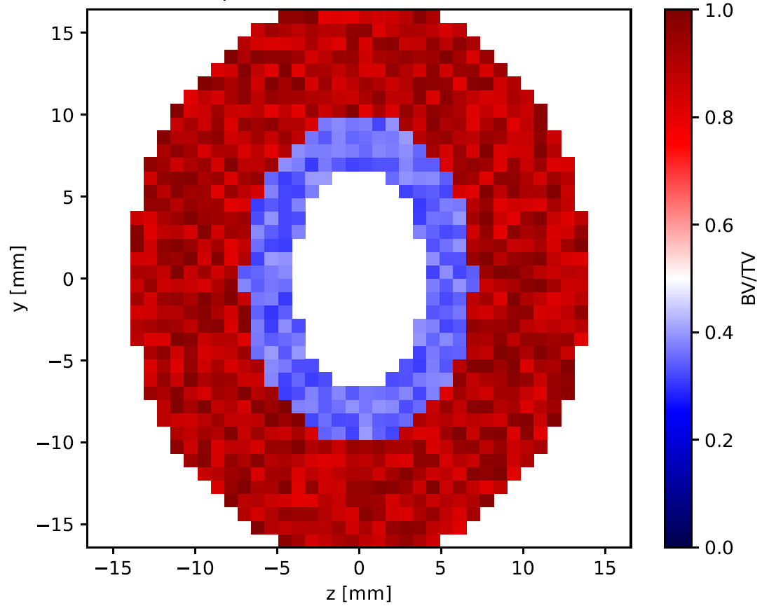
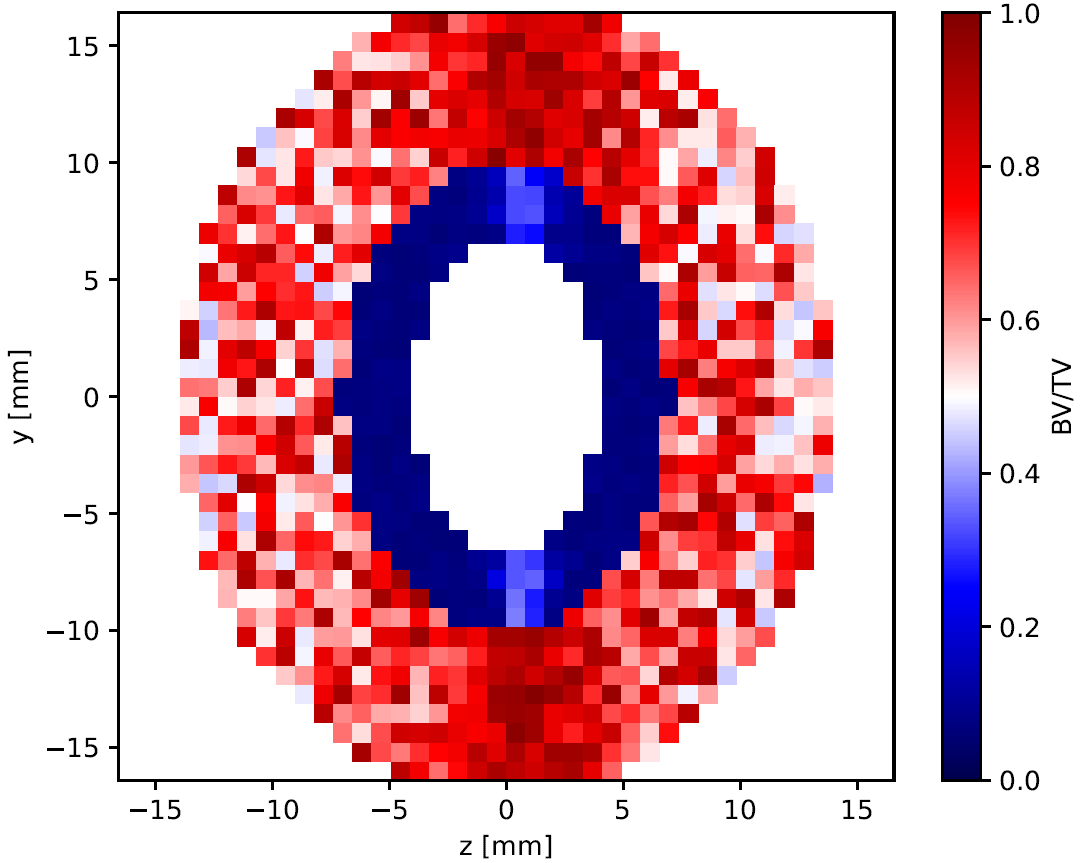
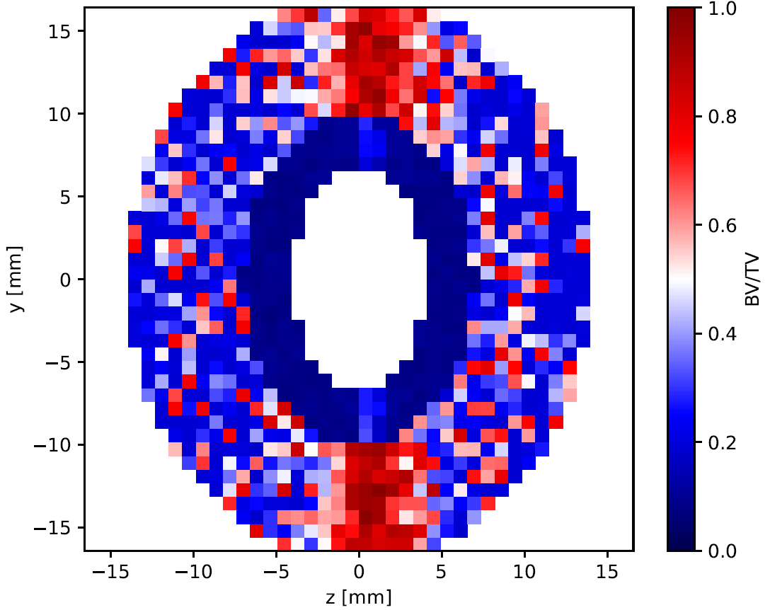
    plt.title(f'BV/TV Distribution - Interval {interval + 1}')
    plt.xlabel('z [mm]')
    plt.ylabel('y [mm]')
    plt.axis('equal')
    plt.tight_layout()
    plt.show()

This will generate a graph showing the evolution of BV/TV in a cross-section over time (initial distribution - microgravity for 1 year - microgravity for 3 year).