Examples
This page demonstrates how to use different bone mineralisation models and visualize their results.
The requirement for running the models is the installation of the bone_models package via running the command
pip install bone_models in the terminal.
Ruffoni Model Example
import matplotlib.pyplot as plt
# import the Ruffoni model
from bone_models.bone_mineralisation_models.models.ruffoni_model import Ruffoni_Model
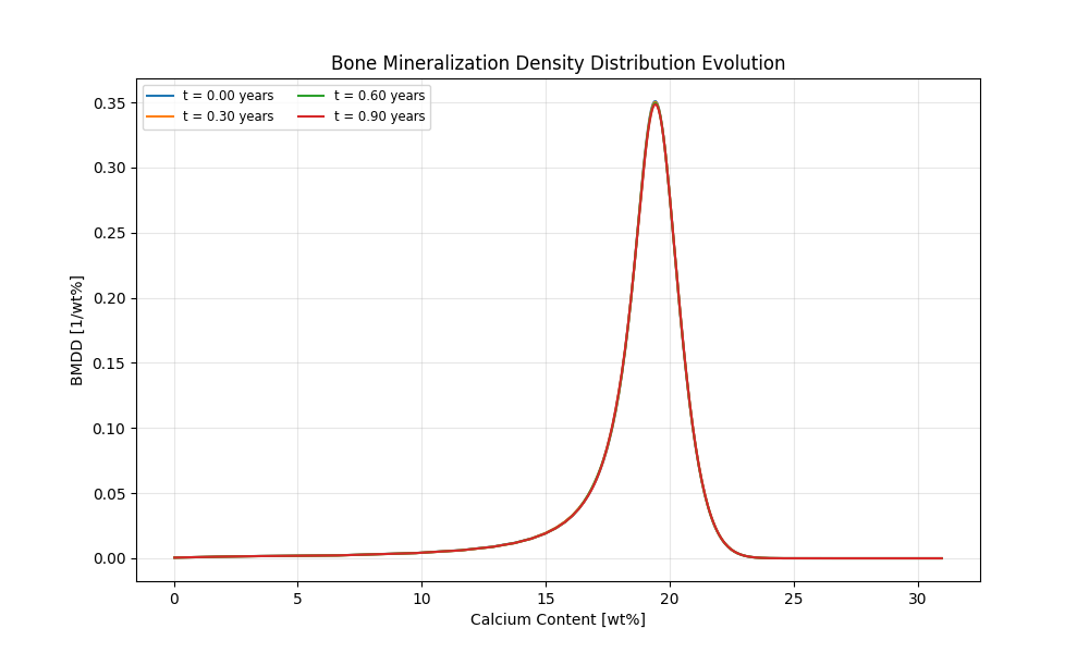
# Initialize the model with a BMDD starting condition
# Simulate homeostatic conditions for 1 year with 500 calcium grid points
model = Ruffoni_Model(simulation_time=1, number_of_grid_points=500, start='BMDD')
# Solve the model, save results every 0.3 years
BMDD_evolution, BV_evolution, time_points = model.solve_for_BMDD(save_interval=0.3)
# Plot results
model.plot_results(BMDD_evolution, BV_evolution, time_points)
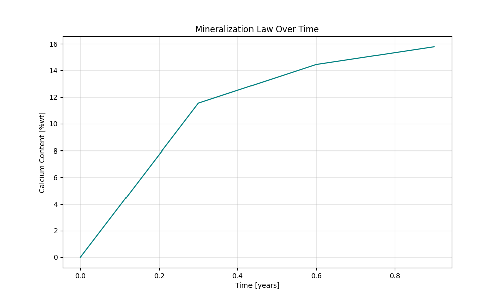
This will generate a graph showing the BMDD evolution in homeostasis over time. You can see minor changes due to numerical effects.
import matplotlib.pyplot as plt
# import the Ruffoni model
from bone_models.bone_mineralisation_models.models.ruffoni_model import Ruffoni_Model
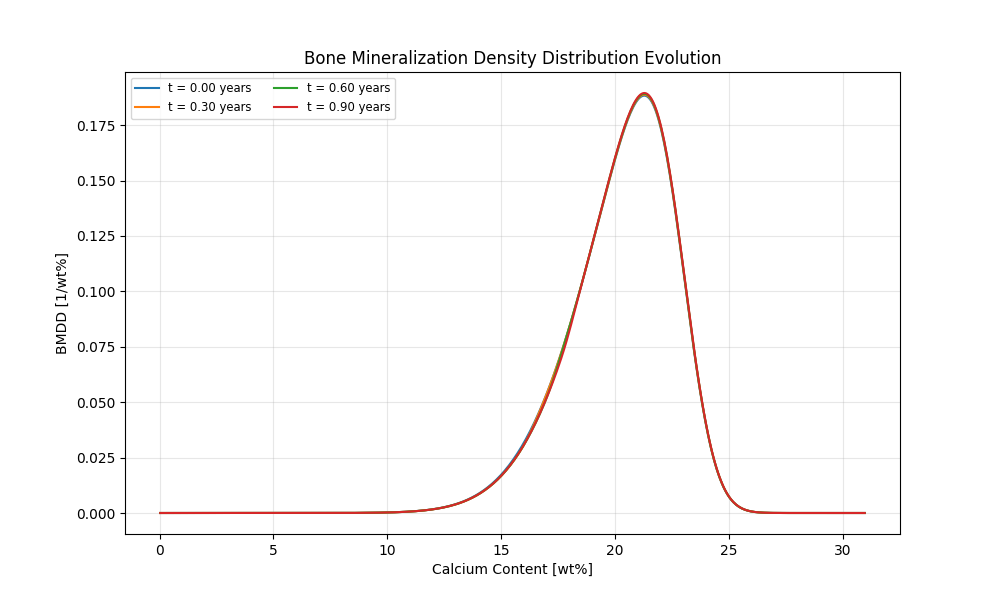
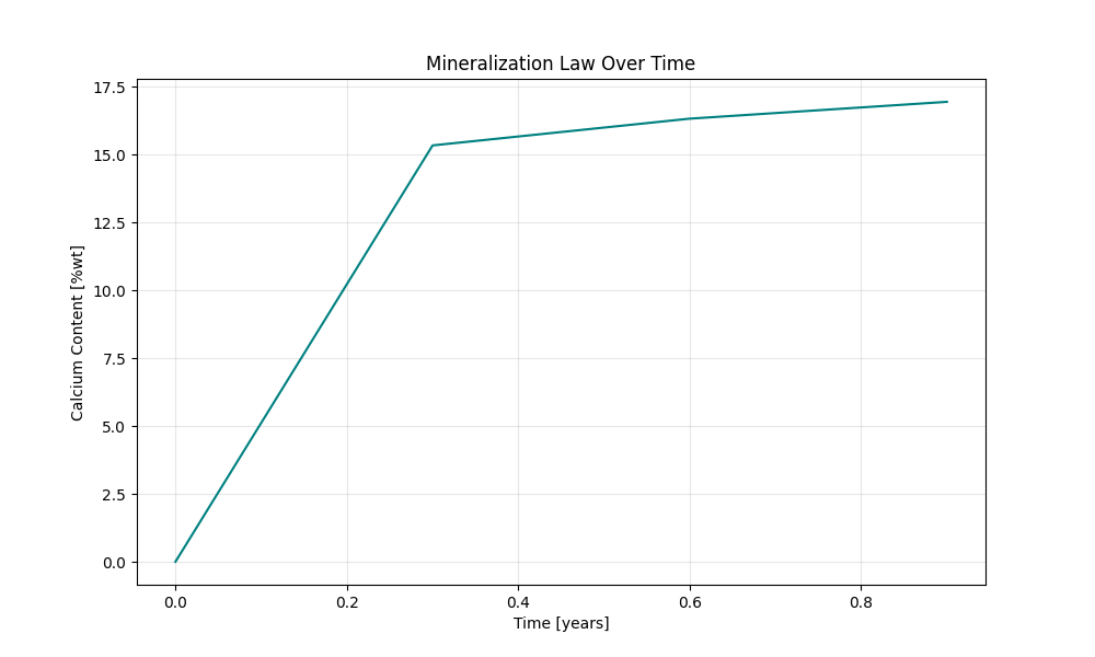
# Initialize the model with a mineralization law
# Simulate homeostatic conditions for 1 year with 500 calcium grid points
model = Ruffoni_Model(simulation_time=1, number_of_grid_points=500, start='mineralization law')
# Solve the model
BMDD_evolution, BV_evolution, time_points = model.solve_for_BMDD(save_interval=0.1)
# Plot results
model.plot_results(BMDD_evolution, BV_evolution, time_points)
This will generate a graph showing the BMDD evolution in homeostasis over time. You can see minor changes due to numerical effects.
Modiz Model Example
from bone_mineralisation_models.models.modiz_model import Modiz_Model
from bone_mineralisation_models.load_cases.modiz_load_cases import Modiz_Load_Case
import matplotlib.pyplot as plt
# Initialise model for several bone volume fractions and save results in lists
load_case = Modiz_Load_Case()
material_density_list, apparent_density_list = [], []
bone_volume_fractions = [0.1, 0.2, 0.3, 0.4, 0.5, 0.6, 0.7, 0.8, 0.9, 0.98]
for bone_volume_fraction in bone_volume_fractions:
# Initialise model with load case ('neutral' - no disease state, only needed for implementation)
# and bone volume fraction between 0 and 1
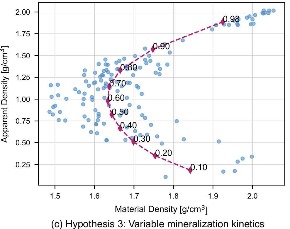
# If called like this, hypothesis 3 (turnover and mineral apposition rate) is tested (default)
model = Modiz_Model(load_case, bone_volume_fraction)
if bone_volume_fraction >= 0.8:
# extend queue for cortical bone
model.parameters.mineralisation.length_of_queue = 45000
material_density, apparent_density = model.calculate_mineral_densities(bone_volume_fraction)
material_density_list.append(material_density)
apparent_density_list.append(apparent_density)
# Plot results vs. experimental data (published in PLOSOne Berli et al. 2017)
plt.figure()
plt.plot(material_density_list, apparent_density_list, marker='d', linestyle='--', label='Model Results')
for i, bvf in enumerate(bone_volume_fractions):
plt.annotate(f'{bvf:.2f}', (material_density_list[i], apparent_density_list[i]))
plt.scatter(experimental_data.iloc[:, 2], experimental_data.iloc[:, 1], label='Experimental Data',)
plt.xlabel(r'Material Density [g/cm$^3$]')
plt.ylabel(r'Apparent Density [g/cm$^3$]')
plt.legend()
plt.show()
This will generate the following plot:
from bone_mineralisation_models.models.modiz_model import Modiz_Model
from bone_mineralisation_models.load_cases.modiz_load_cases import Modiz_Load_Case
import matplotlib.pyplot as plt
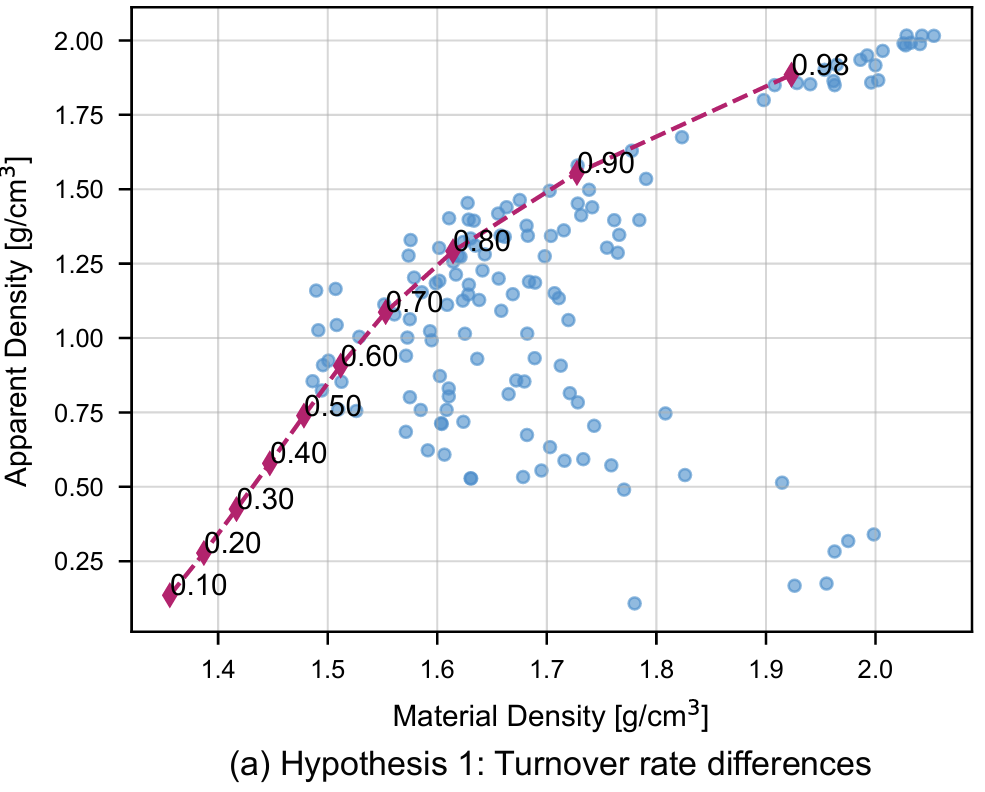
# -------------- Plotting the hypothesis 1 --------------
load_case = Modiz_Load_Case()
material_density_list, apparent_density_list = [], []
bone_volume_fractions = [0.1, 0.2, 0.3, 0.4, 0.5, 0.6, 0.7, 0.8, 0.9, 0.98]
# Test hypothesis 1 (only turnover)
for bone_volume_fraction in bone_volume_fractions:
# Initialise model with load case ('neutral' - no disease state, only needed for implementation)
# and bone volume fraction between 0 and 1
# 'hypothesis' can be either 1, 2.1, 2.2 or 3 (defaults to 3) and determines which hypothesis from the paper is tested
model = Modiz_Model(load_case, bone_volume_fraction, hypothesis=1)
if bone_volume_fraction >= 0.8:
# extend queue for cortical bone
model.parameters.mineralisation.length_of_queue = 45000
material_density, apparent_density = model.calculate_mineral_densities(bone_volume_fraction)
material_density_list.append(material_density)
apparent_density_list.append(apparent_density)
# Plot material and apparent density for both hypotheses
plt.figure()
plt.plot(material_density_list, apparent_density_list, label='Hypothesis 1', marker='d', linestyle='--',)
for i, bvf in enumerate(bone_volume_fractions):
plt.annotate(f'{bvf:.2f}', (material_density_list, apparent_density_list))
plt.scatter(experimental_data.iloc[:, 2], experimental_data.iloc[:, 1], label='Experimental Data',)
plt.xlabel(r'Material Density [g/cm$^3$]')
plt.ylabel(r'Apparent Density [g/cm$^3$]')
plt.legend()
plt.show()
This will generate the following plot: