Examples

This page demonstrates how to use different bone remodeling models and visualize their results. The requirement for running the models is the installation of the bone_models package via running the command pip install bone_models in the terminal.

Lemaire Model Example

import matplotlib.pyplot as plt
# import the Lemaire model
from bone_models.bone_cell_population_models.models import Lemaire_Model
# import the load case - in this case Lemaire_Load_Case_5 that defines a PTH injection scenario
from bone_models.bone_cell_population_models.load_cases.lemaire_load_cases import Lemaire_Load_Case_3

# Define the time span for the simulation
tspan = [0, 140]
# Initialize the load case - in this case the load case determines a PTH injection according to
# Lemaire et al. (2004)
load_case = Lemaire_Load_Case_3()
# Create a model instance with the load case
model = Lemaire_Model(load_case)
# Solve the model and get the solution
# The solution contains time points and cell concentrations (OBp, OBa, OCa)
solution = model.solve_bone_cell_population_model(tspan=tspan)

# Plot the resulting bone cell concentrations
plt.figure()
plt.plot(solution.t, solution.y[0], label='OBp', color='blue', linestyle='--')
plt.plot(solution.t, solution.y[1], label='OBa', color='blue')
plt.plot(solution.t, solution.y[2], label='OCa', color='red')
plt.ticklabel_format(axis='y', style='sci', scilimits=(0,0))
plt.grid(True)
plt.xlabel('Time [days]')
plt.ylabel('Cell Concentrations [pM]')
plt.title('Bone Cell Population Over Time')
plt.legend()
plt.show()

This will generate a graph showing the bone cell concentrations over time.

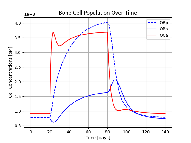
Pivonka Model Example

import matplotlib.pyplot as plt
# import the Pivonka model
from bone_models.bone_cell_population_models.models import Pivonka_Model
# import the load case - in this case Pivonka_Load_Case_1 that defines determines a PTH injection
from bone_models.bone_cell_population_models.load_cases.pivonka_load_cases import Pivonka_Load_Case_1

# Define the time span for the simulation
tspan = [0, 1000]
# Initialize the load case - in this case the load case determines a PTH injection according to Lemaire et al. (2004)
load_case = Pivonka_Load_Case_1()
# Create a model instance with the load case
model = Pivonka_Model(load_case)
# Solve the model and get the solution
# The solution contains time points and cell concentrations (OBp, OBa, OCa)
solution = model.solve_bone_cell_population_model(tspan=tspan)

# Plot the resulting bone cell concentrations
plt.figure()
plt.plot(solution.t, solution.y[0], label='OBp', color='blue', linestyle='--')
plt.plot(solution.t, solution.y[1], label='OBa', color='blue')
plt.plot(solution.t, solution.y[2], label='OCa', color='red')
plt.ticklabel_format(axis='y', style='sci', scilimits=(0,0))
plt.grid(True)
plt.xlabel('Time [days]')
plt.ylabel('Cell Concentrations [pM]')
plt.title('Bone Cell Population Over Time')
plt.legend()
plt.show()

This will generate a graph showing the bone cell concentrations over time.

Scheiner Model Example

from bone_models.bone_cell_population_models.models import Scheiner_Model
from bone_models.bone_cell_population_models.load_cases.scheiner_load_cases import Scheiner_Load_Case
import matplotlib.bone_cell_population_models.pyplot as plt

# Define the time span for the simulation
tspan = [0, 3000]
# Initialize the load case - in this case the load case determines the disuse scenario according to
# Scheiner et al. (2013)
load_case = Scheiner_Load_Case()
# Create a model instance with the load case
model = Scheiner_Model(load_case)
# Solve the model and get the solution
# The solution contains time points, cell concentrations (OBp, OBa, OCa), vascular pores volume fraction,
# bone volume fraction
solution = model.solve_bone_cell_population_model(tspan=tspan)

# Plot the resulting bone cell concentrations
plt.figure()
plt.plot(solution.t, solution.y[0], label='OBp', color='blue', linestyle='--')
plt.plot(solution.t, solution.y[1], label='OBa', color='blue')
plt.plot(solution.t, solution.y[2], label='OCa', color='red')
plt.ticklabel_format(axis='y', style='sci', scilimits=(0,0))
plt.grid(True)
plt.xlabel('Time [days]')
plt.ylabel('Cell Concentrations [pM]')
plt.title('Bone Cell Population Over Time')
plt.legend()
# Plot the resulting vascular pores volume fraction
plt.figure()
plt.plot(solution.t, solution.y[3])
plt.grid(True)
plt.xlabel('Time [days]')
plt.ylabel('Vascular pores volume fraction [%]')
# Plot the resulting bone volume fraction
plt.figure()
plt.plot(solution.t, solution.y[4])
plt.grid(True)
plt.xlabel('Time [days]')
plt.ylabel('Bone volume fraction [%]')
plt.show()

This will generate graphs showing the bone cell concentrations, vascular pore volume fraction and bone volume fraction over time.

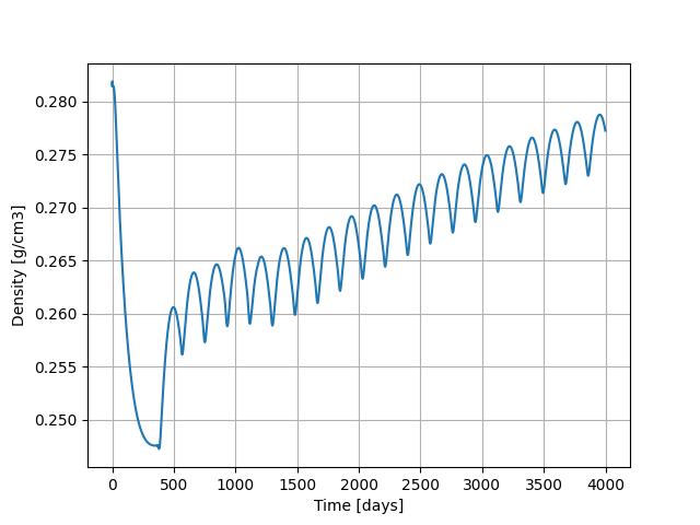
Martinez-Reina Model Example

from bone_models.bone_cell_population_models.models import Martinez_Reina_Model
from bone_models.bone_cell_population_models.load_cases.martinez_reina_load_cases import Martinez_Reina_Load_Case
import matplotlib.pyplot as plt

# Define the time span for the simulation
tspan = [0, 4000]
# Initialize the load case - in this case the load case determines the PMO onset at the simulation start time
# and denosumab injection every half year after 1 year of simulation according to
# Martinez-Reina et al. (2019)
load_case = Martinez_Reina_Load_Case()
# Create a model instance with the load case
model = Martinez_Reina_Model(load_case)
# Solve the model and get the solution.
# The solution contains time points, cell concentrations (OBp, OBa, OCa), vascular pores volume fraction,
# bone volume fraction. Th solution is a list of arrays rather than the result of the solve_ivp function as the
# model has to be solved in multiple steps.
solution = model.solve_bone_cell_population_model(tspan=tspan)
[time, OBp, OBa, OCa, vascular_pore_fraction, bone_volume_fraction] = solution

# Plot the resulting apparent density, calculated each tim the ageing queue is updated
plt.figure()
plt.plot(np.arange(tspan[0], tspan[1], 1), model.bone_apparent_density)
plt.grid(True)
plt.xlabel('Time [days]')
plt.ylabel('Density [g/cm3]')
plt.show()

This will generate a graph showing the apparent density over time.

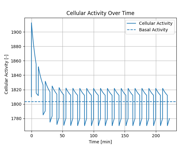
Martonova Model Example

import matplotlib.pyplot as plt
# import the Martonova model
from bone_models.bone_cell_population_models.models import Martonova_Model
# import the load case - in this case Martonova_Hyperparathyroidism that defines a hyperparathyroidism scenario
from bone_models.bone_cell_population_models.load_cases import Martonova_Hyperparathyroidism

# Initialize the load case - in this case the load case determines hyperparathyroidism pulse characteristics according to
# Martonova et al. (2023)
load_case = Martonova_Hyperparathyroidism()
# Create a model instance with the load case
model = Martonova_Model(load_case)
# Solve the model and get the solution
cellular_activity, time, basal_activity, integrated_activity, cellular_responsiveness = model.solve_for_activity()

plt.figure()
plt.plot(time, cellular_activity, label='Cellular Activity')
plt.axhline(y=basal_activity, color='r', linestyle='--', label='Basal Activity')
plt.grid(True)
plt.xlabel('Time [min]')
plt.ylabel('Cellular Activity [-]')
plt.title('Cellular Activity Over Time')
plt.legend()
plt.show()

This will generate graphs showing the cellular activity over time with the basal activity.

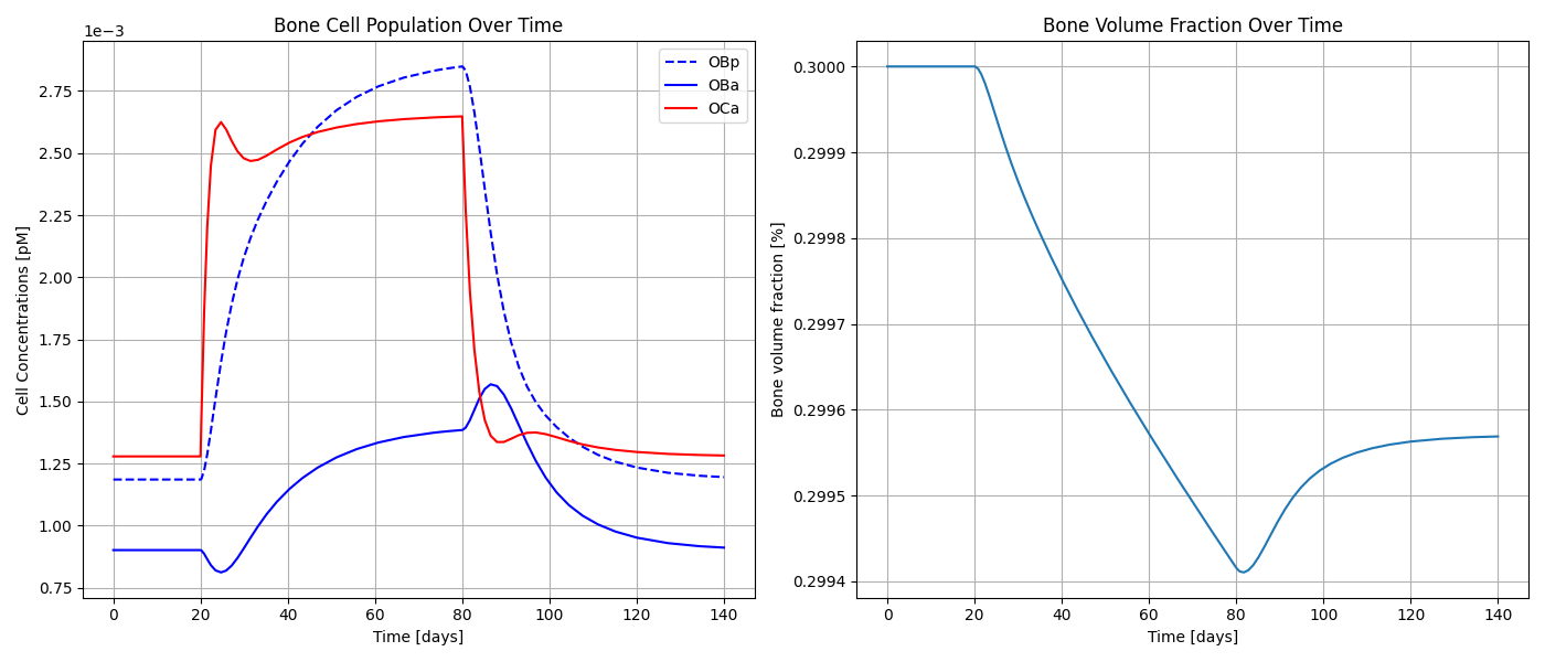
Modiz Model Example

import matplotlib.pyplot as plt
# import the Pivonka model
from bone_models.bone_cell_population_models.models import Modiz_Model
# import the load case - in this case Modiz_Healthy_to_Hyperparathyroidism that defines a healthy to hyperparathyroidism scenario
from bone_models.bone_cell_population_models.load_cases.modiz_load_cases import Modiz_Healthy_to_Hyperparathyroidism

# Define the time span for the simulation
tspan = [0, 140]
# Initialize the load case - in this case the load case determines a healthy to hyperparathyroidism scenario according to Modiz et al. (2025)
load_case = Modiz_Healthy_to_Hyperparathyroidism()
# Create a model instance with the load case
# The model type is 'cellular responsiveness' meaning the cellular responsiveness drives the activation by PTH
# and the calibration type is 'all' meaning calibration includes all disease states
model = Modiz_Model(load_case, model_type='cellular responsiveness', calibration_type='all')
# Solve the model and get the solution
# The solution contains time points and cell concentrations (OBp, OBa, OCa)
solution = model.solve_bone_cell_population_model(tspan=tspan)
# Calculate the bone volume fraction change over time depending on the previously calculated cell concentrations, steady state, and initial bone volume fraction
bone_volume_fraction = model.calculate_bone_volume_fraction_change(solution.t, solution.y, [model.steady_state.OBp, model.steady_state.OBa, model.steady_state.OCa], 0.3)

# Plot the resulting bone cell concentrations
plt.figure()
plt.plot(solution.t, solution.y[0], label='OBp', color='blue', linestyle='--')
plt.plot(solution.t, solution.y[1], label='OBa', color='blue')
plt.plot(solution.t, solution.y[2], label='OCa', color='red')
plt.ticklabel_format(axis='y', style='sci', scilimits=(0,0))
plt.grid(True)
plt.xlabel('Time [days]')
plt.ylabel('Cell Concentrations [pM]')
plt.title('Bone Cell Population Over Time')
plt.legend()
# Plot the resulting bone volume fraction
plt.figure()
plt.plot(solution.t, bone_volume_fraction)
plt.grid(True)
plt.xlabel('Time [days]')
plt.ylabel('Bone volume fraction [%]')
plt.show()

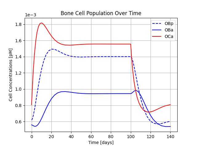
This will generate graphs showing the bone cell dynamics and the bone volume fraction (with initial value 0.3) over time.

Lerebours Model Example

from bone_models.bone_cell_population_models.models.lerebours_model import Lerebours_Model
from bone_models.bone_cell_population_models.load_cases.lerebours_load_cases import Lerebours_Load_Case
import matplotlib.pyplot as plt
import numpy as np

# define the time span for the simulation
tspan = [0, 200]
# initialise the load case (underloading scenario from day 50 to day 150)
load_case = Lerebours_Load_Case()
# define porosity between 0 and 1
porosity = 0.05
# initialise the model instance
model = Lerebours_Model(load_case, porosity)
# solve the model for the given porosity and time span
solution = model.solve_bone_cell_population_model(tspan, porosity)
# time solution contains OBp, OBa, OCp, OCa, vascular porosity, bone volume fraction

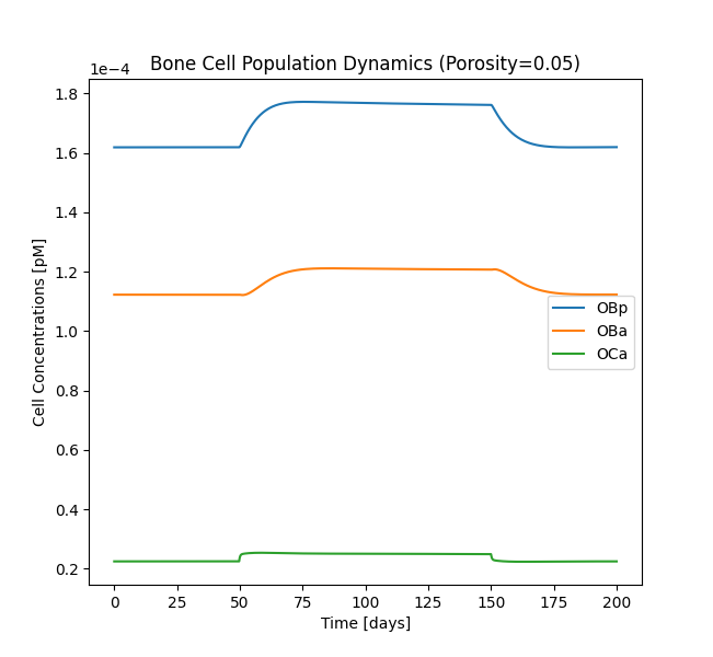
# 1. Bone Cell Population Dynamics
plt.figure(figsize=(10, 6))
plt.plot(solution.t, solution.y[0], label='OBp')
plt.plot(solution.t, solution.y[1], label='OBa')
plt.plot(solution.t, solution.y[3], label='OCa')
plt.xlabel('Time [days]')
plt.ylabel('Cell Concentrations [pM]')
plt.title(f'Bone Cell Population Dynamics (Porosity={porosity})')
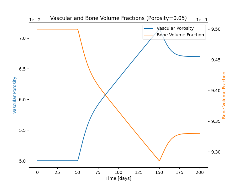
# 2. Vascular Porosity and Bone Volume Fraction
fig, ax1 = plt.subplots(figsize=(10, 6))
ax1.plot(solution.t, solution.y[4], label='Vascular Porosity', color='tab:blue')
ax1.set_xlabel('Time [days]')
ax1.set_ylabel('Vascular Porosity', color='tab:blue')
ax1.ticklabel_format(style='sci', axis='y', scilimits=(0,0))
ax2 = ax1.twinx()
ax2.plot(solution.t, solution.y[5], label='Bone Volume Fraction', color='tab:orange')
ax2.set_ylabel('Bone Volume Fraction', color='tab:orange')
ax2.ticklabel_format(style='sci', axis='y', scilimits=(0,0))
plt.title(f'Vascular and Bone Volume Fractions (Porosity={porosity})')

This will generate graphs showing the cellular activity, vascular fraction and bone volume fraction over time.